Canned PDE Models¶

Base classes for operators.

class hedge.models.HyperbolicOperator¶

A base class for hyperbolic Discontinuous Galerkin operators.

estimate_timestep(discr, stepper=None, stepper_class=None, stepper_args=None, t=None, fields=None)¶: Estimate the largest stable timestep, given a time stepper stepper_class. If none is given, RK4 is assumed.

class hedge.models.Operator¶

A base class for Discontinuous Galerkin operators.

You may derive your own operators from this class, but, at present this class provides no functionality. Its function is merely as documentation, to group related classes together in an inheritance tree.

class hedge.models.TimeDependentOperator¶

A base class for time-dependent Discontinuous Galerkin operators.

Advection¶

class hedge.models.advection.StrongAdvectionOperator¶

flux_types¶

__init__(v, inflow_tag='inflow', inflow_u=hedge.data.TimeConstantGivenFunction(0), outflow_tag='outflow', flux_type='central')¶

max_eigenvalue(t=None, fields=None, discr=None)¶

bind(discr)¶

class hedge.models.advection.WeakAdvectionOperator¶

flux_types¶

__init__(v, inflow_tag='inflow', inflow_u=hedge.data.TimeConstantGivenFunction(0), outflow_tag='outflow', flux_type='central')¶

max_eigenvalue(t=None, fields=None, discr=None)¶

bind(discr)¶

class hedge.models.advection.VariableCoefficientAdvectionOperator(dimensions, advec_v, bc_u_f='None', flux_type='central', diffusion_coeff=None, diffusion_scheme=<hedge.second_order.CentralSecondDerivative object at 0x542e110>)¶

Bases: hedge.models.HyperbolicOperator

A class for space- and time-dependent DG advection operators.

Parameters:	advec_v – Adheres to the `hedge.data.ITimeDependentGivenFunction` interfacer and is an n-dimensional vector representing the velocity. bc_u_f – Adheres to the `hedge.data.ITimeDependentGivenFunction` interface and is a scalar representing the boundary condition at all boundary faces.

Optionally allows diffusion.

flux_types¶

__init__(dimensions, advec_v, bc_u_f='None', flux_type='central', diffusion_coeff=None, diffusion_scheme=<hedge.second_order.CentralSecondDerivative object at 0x542e110>)¶

max_eigenvalue(t, fields=None, discr=None)¶

bind(discr, sensor=None)¶

$n$ -dimensional Calculus¶

class hedge.models.nd_calculus.GradientOperator(dimensions)¶

Bases: hedge.models.Operator

__init__(dimensions)¶

bind(discr)¶

class hedge.models.nd_calculus.DivergenceOperator(dimensions, subset=None)¶

Bases: hedge.models.Operator

__init__(dimensions, subset=None)¶

bind(discr)¶

Waves¶

class hedge.models.wave.StrongWaveOperator(c, dimensions, source_f=None, flux_type='upwind', dirichlet_tag=TAG_ALL, dirichlet_bc_f=None, neumann_tag=TAG_NONE, radiation_tag=TAG_NONE)¶

Bases: hedge.models.HyperbolicOperator

This operator discretizes the wave equation $\partial_t^2 u = c^2 \Delta u$ .

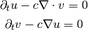
To be precise, we discretize the hyperbolic system

$\partial_t u - c \nabla \cdot v = 0 \partial_t v - c \nabla u = 0$

The sign of $v$ determines whether we discretize the forward or the backward wave equation.

$c$ is assumed to be constant across all space.

__init__(c, dimensions, source_f=None, flux_type='upwind', dirichlet_tag=TAG_ALL, dirichlet_bc_f=None, neumann_tag=TAG_NONE, radiation_tag=TAG_NONE)¶

bind(discr)¶

class hedge.models.wave.VariableVelocityStrongWaveOperator(c, dimensions, source=None, flux_type='upwind', dirichlet_tag=TAG_ALL, neumann_tag=TAG_NONE, radiation_tag=TAG_NONE, time_sign=1, diffusion_coeff=None, diffusion_scheme=<hedge.second_order.CentralSecondDerivative object at 0x3dbea50>)¶

Bases: hedge.models.HyperbolicOperator

This operator discretizes the wave equation $\partial_t^2 u = c^2 \Delta u$ .

To be precise, we discretize the hyperbolic system

$\partial_t u - c \nabla \cdot v = 0 \partial_t v - c \nabla u = 0$

__init__(c, dimensions, source=None, flux_type='upwind', dirichlet_tag=TAG_ALL, neumann_tag=TAG_NONE, radiation_tag=TAG_NONE, time_sign=1, diffusion_coeff=None, diffusion_scheme=<hedge.second_order.CentralSecondDerivative object at 0x3dbea50>)¶

c is assumed to be positive and conforms to the hedge.data.ITimeDependentGivenFunction interface.

source also conforms to the hedge.data.ITimeDependentGivenFunction interface.

bind(discr, sensor=None)¶

Electromagnetism¶

class hedge.models.em.MaxwellOperator(epsilon, mu, flux_type, bdry_flux_type=None, pec_tag=TAG_ALL, pmc_tag=TAG_NONE, absorb_tag=TAG_NONE, incident_tag=TAG_NONE, incident_bc=None, current=None, dimensions=None)¶

Bases: hedge.models.HyperbolicOperator

A 3D Maxwell operator which supports fixed or variable isotropic, non-dispersive, positive epsilon and mu.

Field order is [Ex Ey Ez Hx Hy Hz].

__init__(epsilon, mu, flux_type, bdry_flux_type=None, pec_tag=TAG_ALL, pmc_tag=TAG_NONE, absorb_tag=TAG_NONE, incident_tag=TAG_NONE, incident_bc=None, current=None, dimensions=None)¶

Parameters:

Parameters:	flux_type – can be in [0,1] for anything between central and upwind, or “lf” for Lax-Friedrichs epsilon – can be a number, for fixed material throughout the computation domain, or a TimeConstantGivenFunction for spatially variable material coefficients mu – can be a number, for fixed material throughout the computation domain, or a TimeConstantGivenFunction for spatially variable material coefficients

flux_type – can be in [0,1] for anything between central and upwind, or “lf” for Lax-Friedrichs
epsilon – can be a number, for fixed material throughout the computation domain, or a TimeConstantGivenFunction for spatially variable material coefficients
mu – can be a number, for fixed material throughout the computation domain, or a TimeConstantGivenFunction for spatially variable material coefficients

bind(discr, **extra_context)¶: Convert the abstract operator template into compiled code.

partial_to_eh_subsets()¶: Helps find the indices of the E and H components, which can vary depending on number of dimensions and whether we have a full/TE/TM operator.

split_eh(w)¶: Splits an array into E and H components

assemble_eh(e=None, h=None, discr=None)¶: Combines separate E and H vectors into a single array.

get_eh_subset()¶: Return a 6-tuple of bool objects indicating whether field components are to be computed. The fields are numbered in the order specified in the class documentation.

max_eigenvalue(t, fields=None, discr=None)¶: Return the largest eigenvalue of Maxwell’s equations as a hyperbolic system.

class hedge.models.em.TMMaxwellOperator(epsilon, mu, flux_type, bdry_flux_type=None, pec_tag=TAG_ALL, pmc_tag=TAG_NONE, absorb_tag=TAG_NONE, incident_tag=TAG_NONE, incident_bc=None, current=None, dimensions=None)¶

Bases: hedge.models.em.MaxwellOperator

A 2D TM Maxwell operator with PEC boundaries.

Field order is [Ez Hx Hy].

class hedge.models.em.TEMaxwellOperator(epsilon, mu, flux_type, bdry_flux_type=None, pec_tag=TAG_ALL, pmc_tag=TAG_NONE, absorb_tag=TAG_NONE, incident_tag=TAG_NONE, incident_bc=None, current=None, dimensions=None)¶

Bases: hedge.models.em.MaxwellOperator

A 2D TE Maxwell operator.

Field order is [Ex Ey Hz].

class hedge.models.em.TE1DMaxwellOperator(epsilon, mu, flux_type, bdry_flux_type=None, pec_tag=TAG_ALL, pmc_tag=TAG_NONE, absorb_tag=TAG_NONE, incident_tag=TAG_NONE, incident_bc=None, current=None, dimensions=None)¶

Bases: hedge.models.em.MaxwellOperator

A 1D TE Maxwell operator.

Field order is [Ex Ey Hz].

class hedge.models.em.SourceFree1DMaxwellOperator(epsilon, mu, flux_type, bdry_flux_type=None, pec_tag=TAG_ALL, pmc_tag=TAG_NONE, absorb_tag=TAG_NONE, incident_tag=TAG_NONE, incident_bc=None, current=None, dimensions=None)¶

Bases: hedge.models.em.MaxwellOperator

A 1D TE Maxwell operator.

Field order is [Ey Hz].

Electromagnetism with PMLs¶

class hedge.models.pml.AbarbanelGottliebPMLMaxwellOperator(*args, **kwargs)¶

Bases: hedge.models.em.MaxwellOperator

Implements a PML as in

[1] S. Abarbanel and D. Gottlieb, “On the construction and analysis of absorbing layers in CEM,” Applied Numerical Mathematics, vol. 27, 1998, S. 331-340. (eq 3.7-3.11)

[2] E. Turkel and A. Yefet, “Absorbing PML boundary layers for wave-like equations,” Applied Numerical Mathematics, vol. 27, 1998, S. 533-557. (eq. 4.10)

[3] Abarbanel, D. Gottlieb, and J.S. Hesthaven, “Long Time Behavior of the Perfectly Matched Layer Equations in Computational Electromagnetics,” Journal of Scientific Computing, vol. 17, Dez. 2002, S. 405-422.

Generalized to 3D in doc/maxima/abarbanel-pml.mac.

assemble_ehpq(e=None, h=None, p=None, q=None, discr=None)¶

split_ehpq(w)¶

bind(discr, coefficients)¶

coefficients_from_boxes(discr, inner_bbox, outer_bbox=None, magnitude=None, tau_magnitude=None, exponent=None, dtype=None)¶

coefficients_from_width(discr, width, magnitude=None, tau_magnitude=None, exponent=None, dtype=None)¶

class hedge.models.pml.AbarbanelGottliebPMLTEMaxwellOperator(*args, **kwargs)¶: Bases: hedge.models.em.TEMaxwellOperator, hedge.models.pml.AbarbanelGottliebPMLMaxwellOperator

class hedge.models.pml.AbarbanelGottliebPMLTMMaxwellOperator(*args, **kwargs)¶: Bases: hedge.models.em.TMMaxwellOperator, hedge.models.pml.AbarbanelGottliebPMLMaxwellOperator

Diffusion¶

class hedge.models.diffusion.DiffusionOperator(dimensions, diffusion_tensor=None, dirichlet_bc=hedge.data.TimeConstantGivenFunction(0), dirichlet_tag='dirichlet', neumann_bc=hedge.data.TimeConstantGivenFunction(0), neumann_tag='neumann', scheme=<hedge.second_order.CentralSecondDerivative object at 0x4f035d0>)¶

Bases: hedge.models.TimeDependentOperator, hedge.models.poisson.LaplacianOperatorBase

__init__(dimensions, diffusion_tensor=None, dirichlet_bc=hedge.data.TimeConstantGivenFunction(0), dirichlet_tag='dirichlet', neumann_bc=hedge.data.TimeConstantGivenFunction(0), neumann_tag='neumann', scheme=<hedge.second_order.CentralSecondDerivative object at 0x4f035d0>)¶

bind(discr)¶: Return a BoundPoissonOperator.

Poisson¶

class hedge.models.poisson.PoissonOperator(dimensions, diffusion_tensor=None, dirichlet_bc=hedge.data.ConstantGivenFunction(0), dirichlet_tag='dirichlet', neumann_bc=hedge.data.ConstantGivenFunction(0), neumann_tag='neumann', scheme=<hedge.second_order.LDGSecondDerivative object at 0x4f03450>)¶

Bases: hedge.models.Operator, hedge.models.poisson.LaplacianOperatorBase

Implements the Local Discontinuous Galerkin (LDG) Method for elliptic operators.

See P. Castillo et al., Local discontinuous Galerkin methods for elliptic problems”, Communications in Numerical Methods in Engineering 18, no. 1 (2002): 69-75.

__init__(dimensions, diffusion_tensor=None, dirichlet_bc=hedge.data.ConstantGivenFunction(0), dirichlet_tag='dirichlet', neumann_bc=hedge.data.ConstantGivenFunction(0), neumann_tag='neumann', scheme=<hedge.second_order.LDGSecondDerivative object at 0x4f03450>)¶

bind(discr)¶: Return a BoundPoissonOperator.

class hedge.models.poisson.BoundPoissonOperator(poisson_op, discr)¶

Returned by PoissonOperator.bind().

__call__(u)¶

prepare_rhs(rhs)¶

Prepare the right-hand side for the linear system op(u)=rhs(f).

In matrix form, LDG looks like this:

$Mv = Cu + g Mf = Av + Bu + h$

where v is the auxiliary vector, u is the argument of the operator, f is the result of the grad operator, g and h are inhom boundary data, and A,B,C are some operator+lifting matrices.

$M f = A M^{-1}(Cu + g) + Bu + h$

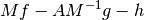
so the linear system looks like

$M f = A M^{-1} Cu + A M^{-1} g + Bu + h M f - A M^{-1} g - h = (A M^{-1} C + B)u (*)$

So the right hand side we’re putting together here is really

$M f - A M^{-1} g - h$

Note

Resist the temptation to left-multiply by the inverse mass matrix, as this will result in a non-symmetric matrix, which (e.g.) a conjugate gradient Krylov solver will not take well.

Canned PDE Models¶

Advection¶

-dimensional Calculus¶

Waves¶

Electromagnetism¶

Electromagnetism with PMLs¶

Diffusion¶

Poisson¶

Gas Dynamics¶

$n$ -dimensional Calculus¶